So finally I got my hands on this gadget - LEAP MOTION.
Those who are not familiar with Leap Motion -
"The Leap Motion Controller senses how you naturally move your hands and lets you use your computer in a whole new way. Point, wave, reach, grab. Pick something up and move it. Do things you never dreamed possible."
So this tiny device, which comes with a huge price tag of $127 (India), senses your fingers and lets you interact with your computer in a whole new way. I made a test demo video embedded below to show how this interaction takes place.
I tried testing it on Ubuntu 12.04 LTS and Windows 7 Ultimate. It failed to run on my 12.04 LTS (need to check it why?) and after going through some threads I came across that it works fine on 12.10 and 13.04. I spent quite some time running it on Shivanshu's Ubuntu (12.10 perhaps). It was working fine, but required good lighting for functioning accurately. But somehow Leap is not polished for Linux compared to Windows. On Windows it gives you more options for Tracking Priority (Balanced, Precision, High Speed) and you can even re-calibrate your device.
The Airspace Store kinda sucks for both Windows and Linux (Too few apps).
Now coming to the Leap SDK for Developers.
Well Leap surely has wooed us developers by providing SDK in Python and Javascript (both work really well). I can see Pygame hooked to leap in near future. But the star attraction is definitely the Javascript SDK. You can see countless possibilities of using Leap along with WebGL.
Here are some of the open source projects you should look forward too if you planning to hack your Leap:
GSoC finally comes to an end.
It was a wonderful experience.
My projects and docs are available on my repo.
It was an awesome experience going through the wonderful projects of other pythonistas.
PS: I will get a bit informal in today's report. Do forgive me for that.
Past 14 days have given me the best coding experience of my lifetime. After doing rigorous research I had formalized my problem statement earlier and started working on it. I realised the true intricacies in my problem when I started searching for methods by which phase change simulations are implemented. I had to change my earlier timeline and jump to my project problem directly. This field is a relatively new field and the algorithms have been developed surrounding the legacy SIMPLE algorithm by Patankar. From Brent, A.D., Voller, V.R. and Reid, K.J.(1988) to Chakraborty, P R and Dutta, P
(2011), people have developed the enthalpy update scheme for accounting phase change keeping Patankar's algorithm as the base. I was familiar with SIMPLE algorithm earlier so I have developed a phase change solver for SfePy using Semi-Implicit Method for Pressure Linked Equations (Revised) or SIMPLER algorithm which is much more robust than SIMPLE algorithm.
The solver code is located here.
Download test problem file here.
Run python brent_test.py
You will get an output dir containing the vtk files which can be viewed using ./postproc.py <file>.vtk
Sample:
The entire group can be loaded in Paraview and you can get the animation.
The code has been validated for the melting gallium experiment performed by Gau and Viskanta(1986) & Brent et al.(1988).
You can see that the code is following the trend and the difference is due to the slight change in thermophysical properties of Gallium taken in the code which might be different while performing the experiments.
Here are some videos of the final result I obtained using the new solver I developed for Phase Change Effect Simulation.
A more detailed blogpost will follow soon.
Right now just enjoy the videos. :)
The final problem accounting convection-diffusion along with phase change has
been defined below along with the governing equations and validation case
studies.
Problem
Heat transfer in the processing of materials involving solid-liquid phase
transformations (melting and solidification) is commonplace in such fields
as metallurgy, crystal growth from melts and solutions, purification of
materials, and solidification of metals. The associated density gradients
in a gravitational field can induce natural convection flows. Convection
in the liquid phase influences the process in two different ways, one of
which is beneficial and the other of which can be detrimental. During
melting convection increases the overall transport rate and, hence, the
growth rate of the new phase, which is desirable. On the other hand, during
solidification convection decreases the growth of the new phase and also seems to
affect the morphology of the solid-liquid interface adversely. The nature
of the solid is largely determined by what occurs in the vicinity of the
solid-liquid interface. The heat release (absorption), density change, and other
processes that take place in the vicinity of the transformation front result in
nonuniformities along the front that cause its shape to change. The resulting
density gradients in the liquid generate buoyancy-driven convection that
can affect the transport of heat, constituent chemicals, and the growth
rate.
The physical domain considered is shown in the figure. The vertical side
walls of the enclosure are maintained at uniform temperatures, while the
connecting horizontal walls are adiabatic. The govering equations are
written for the entire domain assuming constant thermophysical properties,
Boussinesq approximation, laminar, incompressible, and Newtonian
two-dimensional flow. The solid-liquid interface motion due to volume
change upon melting or solidification is neglected through the assumption
.
Nomenclature
Density
kg/m
Viscosity
Pa.s
Specific heat capacity
J/kg.K
Thermal conductivity
W/m.K
Thermal expansion coefficient
1/K
Latent heat of fusion
J/kg
Enthalpy
J/kg
Volume fraction
Temperature
C
Time
s
Velocity
m/s
Pressure
Pa
Source term
m/s
Subscript
Liquid
Solid
Reference
Effective
Hot
Cold
Initial
Melting
Governing Equations
The continuum relations:
1. Continuity
2. Momentum
Now the key lies in modelling the source term. The coefficient
which should tend to 0 as the liquid volume fraction
approaches
unity, and should become a large negative number to anhilate the motion in the fluid
region at .
Whereas these asymtotic conditions can be satisfied by several functions, we
adopt the suggestion of Brent et al. :
where
2. Energy
Writing a general equation for conservation of thermal energy for all the zones in the
domain is facilitated by focusing on an element undergoing phase change. Below
are the energy equation of solid and liquid phases under the thermal equilibrium
condition :
Solid
Liquid
where
and
are the interphase energy terms, having the same magnitude but being opposite in
sign.
A single governing enthalpy equation results:
where
The latent heat content of the element is due to the fraction of liquid converted
to, or from, the corresponding quantity of solid. Hence we write
where L is the latent heat of fusion.
The zones where ,
the entire element is in the liquid state and
.
The zones where ,
the entire element is in the liquid state and
.
It is the elements undergoing phase change at
, where
varies between 0
and 1. Substituting
and
in equation we get
Boundary Conditions
Left
wall
Right
wall
Top
Bottom
Left
wall
Right
wall
Walls
Validation Cases
Melting Gallium : Gau and Viskanta
Melting Gallium : Brent et al.
Melting Calcium chloride : Zivkovic and Fujii
References
Zivkovic, B., Fujii, I., 2001. “An Analysis of Isothermal Phase
Change of Phase Change Material within Rectangular and Cylindrical
Containers”. Solar Energy, 70, pp. 51-61.
Brent, A.D., Voller, V.R., Reid, K.J.,
1988. “Enthalpy-porosity Technique for Modeling Convection-diffusion
Phase Change: Application to the Melting of a Pure Metal”. NumericalHeat Transfer, 13(3), pp. 297-318.
Gau, C., Viskanta, R., 1986. “Melting and Solidification of a Pure Metal
on a Vertical Wall”. Journal of Heat Transfer, 108(1), pp. 174-181.
Rajeev, K., Das, S., 2010. “A Numerical Study for Inward Solidification
of a Liquid Contained in Cylindrical and Spherical Vessel”. ThermalScience, 14(2), pp. 365-372.
Vreeman, C. J., Krane, M. J. M., Incropera, F. P. , 2000. “The Effect of
Free-Floating Dendrites and Convection on Macrosegregation in Direct
Chill Cast Aluminum Alloys. Part 1: Model Development”. Int. J. HeatMass Transfer, 43, pp. 677-686.
Flemings, M. C., 1974. Solidification Processing. McGraw-Hill, New
York.
Kumar, A., Walker, M. J., Sundarraj, S., Dutta, P., 2011. “Grain
Floatation During Equiaxed Solidification of an Al-Cu Alloy in a
Side-Cooled Cavity: Part II-Numerical Studies”. Metallurgical andMaterials Transactions, 42(B), pp. 783-799.
Voller, V.R., 2006. Handbook of Numerical Heat Transfer, 2nd ed..
Wiley, New York, NY, pp. 593-622.
- Firstly after huge amount of discussions we finalised the Navier-Stokes solver and have started development on it.
- In parallel, working on the coupled convective-diffusive problem that I have selected: Laminar Heat Transfer to a Steady Couette Flow
between parallel plates. Where first the Navier Stokes Equation will be solved to determine the velocity and pressure field and then that will be used to determine the temperature field using the Energy Equation.
- I have also added new examples:
Steady Axial convection and diffusion in parabolic flow with maximum velocity U in an insulated pipe.
This week kicked off with the hunt for a robust Navier-Stokes solver for SfePy.
I went through huge amount of resources.
To summarise the journey:
For our Navier-Stokes currently we use the Newton method with
backtracking line-search. in OpenFoam and most of the CFD code the
linearization approach is based on Patankar's SIMPLE algorithm.[1][2]
I talked to my professor who told me that SIMPLE is used in commercial softwares like FLUENT too.
I found few papers which tells us some other approaches:
2D Navier-Stokes solver implemented as a Python package with Python
modules and C++ extension modules. It uses the finite difference method
on a uniform, rectangular grid. It handles single- and two-phase
incompressible, Newtonian, laminar flow with obstacles. -https://code.google.com/p/kmkns/
This
is everything I could harness this week. There is a lot of things to take care to lock the final solver to be used which I would do the current week. Also I am currently narrowing down and rigorously
searching a way to implementing SIMPLE in the FE context.
On a side note I have also been working on a SfePy version for Python 3 and benchmarking the simulation results.
After developing more understanding of SfePy I moved towards implementation.
The first phase of my project involved implementation of convective-diffusive equations.
So with the help of my mentor R (Robert. He is awesome!), energy equations were implemented.
The sample problem taken was:
r"""
Steady Axial convection and diffusion in slug flow with velocity :math:`U _0`
in an insulated pipe.
It is subjected to specified temperature at the entry and exit lengths -
:math:`T _0 for x \leqslant 0`
:math:`T _1 for x \geqslant L`
:math:`\alpha \frac {\partial T}{\partial n} = 0 on the lateral surface of the pipe`
Find :math:`T` such that:
.. math::
\int_{\Omega} c \nabla v \cdot \nabla T
=
- \int_{\Omega_L} (\vec{u} \cdot \nabla T) v
"""
Now the results were pretty interesting :
The results were in accordance with the Peclet number graph which predicts the Temperature distribution in a convective-diffusive case.
We have realised that a robust Navier-Stokes solver is necessary for the project compared to the present solver so our next task is to get that in place and then move ahead with the coupling of the two equations.
I am Ankit and this week I kickstarted my GSoC 2013 Project - Enhancing the solver to simulate solid-liquid phase change phenomenon in convective-diffusive situations. I am a dual-degree undergrad pursuing my masters in phase-change material simulation.
Previously I had worked on the post processor of Abaqus, a
commercial software, in my internship and always dreamed of working on a
solver. Surely it was an honour when I was given a chance to work on SfePy as my GSoC project.
"Briefly, SfePy is a software for solving systems of coupled partial differential
equations (PDEs) by the finite element method in 2D and 3D. It can be viewed
both as black-box PDE solver, and as a Python package which can be used for
building custom applications. The word 'simple' means that complex FEM
problems can be coded very easily and rapidly."
This week ended with:
Finalizing the weak form of the equations to be implemented.
Tinkering with the examples and code-base to know the entire architecture which is very modular and powerful.
I realised that lots of challenges are awaiting ahead, but the interesting part is that SfePy falls under the umbrella organisation - Python Software Foundation
Today is the most exciting day of my 'FOSSDev - Free and Open Source Software Development' history as Robert closed Issue #167 of the SfePy project. Those who are hearing about this project for the first time well SfePy is a software for solving systems of coupled partial differential equations (PDEs) by the finite element method in 2D and 3D. Do try it someday! :)
I came across this project a few months back and was very excited to contribute in it. For past three years I have been working on projects which had a very restricted circle and it was high time to find a greater purpose. Finally I feel as if I have taken a small step in a new direction filled with a new confidence because someone once said -
"That's one small step for a man, a giant leap for mankind."
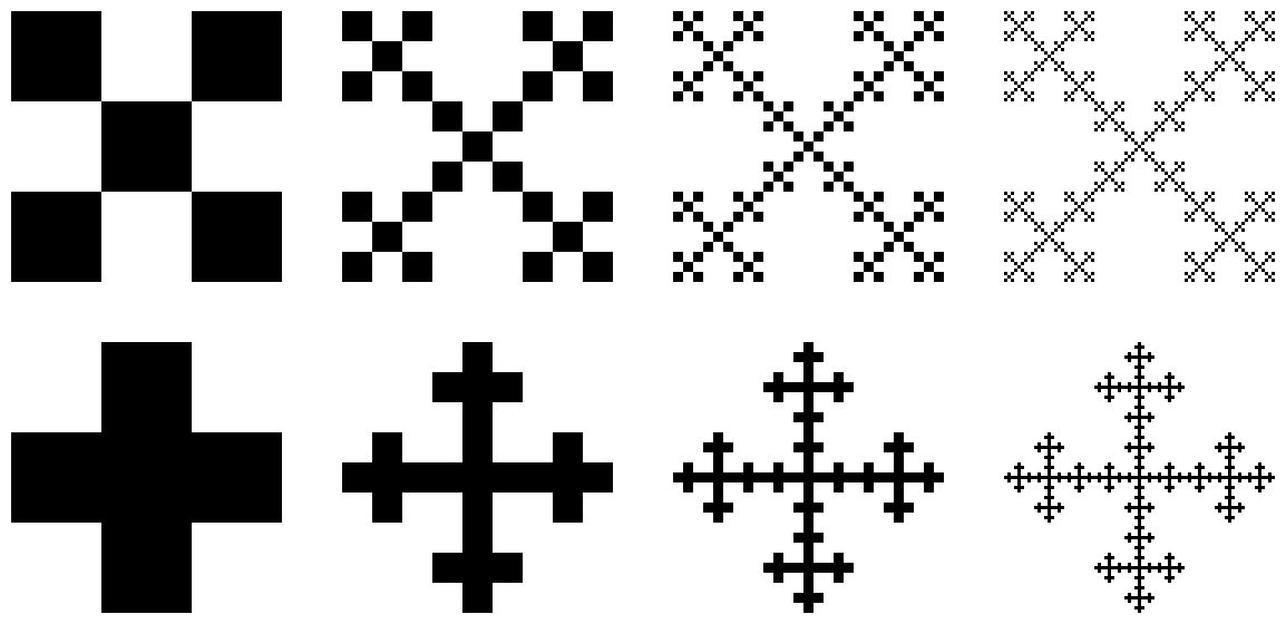
Vicsek fractal is also known as Vicsek snowflake or box fractal.
The basic square is decomposed into nine smaller squares in the 3-by-3 grid. The four squares at the corners and the middle square are left, the other squares being removed. The process is repeated recursively for each of the five remaining subsquares.
An alternative construction (shown below in the left image) is to remove the four corner squares and leave the middle square and the squares above, below, left and right of it. The two constructions produce identical limiting curves, but one is rotated by 45 degrees with respect to the other.
The Vicsek fractal is the set obtained at the limit of this procedure. The Hausdorff dimension of this fractal is log 5/log 3 ≈ 1.46497. (Source : Wikipedia)
Moving ahead ...
I created Viscek fractal using python module tkinter and its inbuilt canvas. A simple python 2.x code to visualize it is given below ...